This talk is part 3 of a series on Experimental Design tutorials given at GemCity ML.
It based strongly on Dr. David Sweet’s book called “Experimentation for Engineers” (Sweet (2022))
Experimental Design Tutorials:
A/B Testing
Multi-arm Bandints
Bayesian Optimization
Why Design an Experiment
It cost money to run an experiment!
It also cost money to train algorithms and implement algorithms.
GPU time is expensive, if you can train and run on a CPU you can save a lot of money.
How do you know if you can reduce sample size and runtime?
With Math!
There are mathematical models you can use to identify what is the number of sample you need to get good results. (see A/B testing)
In addition, not knowing how to adjust your experiment to meet the risk, can cost you your job and/or the company a lot of money.
When, Google debuted their Bard, it failed. It cost the company $100B in valuation. This was a high risk demo.
You need to know how to adjust your experiments for the risk!
This is where design experimentation comes in. How does one adjust for risk while reducing the cost of running the experiment.
One way to reduce cost and risk is to set-up an A/B Test, but that is only good for two variables: A and B.
How do you design an experiment when you have lots of variables.
This is were Bayesian Optimization comes in.
Bayesian Optimization: BO
Bayesian optimization is a sequential design strategy for global optimization of black-box functions that does not assume any functional forms.
How is this Machine Learning?
Machine Learning Models have multiple hyper-parameters that need to be optimized.
The model is a black-box function.
Training a ML model can take hours to weeks per configuration.
You want to quickly find the hyper-parameters that work well and before this decade ends!
Bayesian Optimization: BO
Bayesian optimization is a sequential design strategy for global optimization of black-box functions that does not assume any functional forms.
How is this useful for Software Engineering?
Say you need to speed up the a web application. You can control seven parameters. However, each experiment will take an hour to run. (Sweet (2022))
BO: would take 2 days to run!
Yes, it is that good.
Grid: at 1/10 span spacing would take 10**7/24 = 417,000 days
It is worth the time to set up a Bayesian Optimization algorithm!
Software Engineering Example
The following example is from “Experimentation for Engineers”, by Dr. Sweet (Sweet (2022)).
Outline of Talk
Optimize a single parameter
Model the Response Surface
Optimize over the Acquisition Function
Expected result - uncertainty (aka Lower Confidence Bound (LCB))
Pull it all together for a multi variable Bayesian Optimization
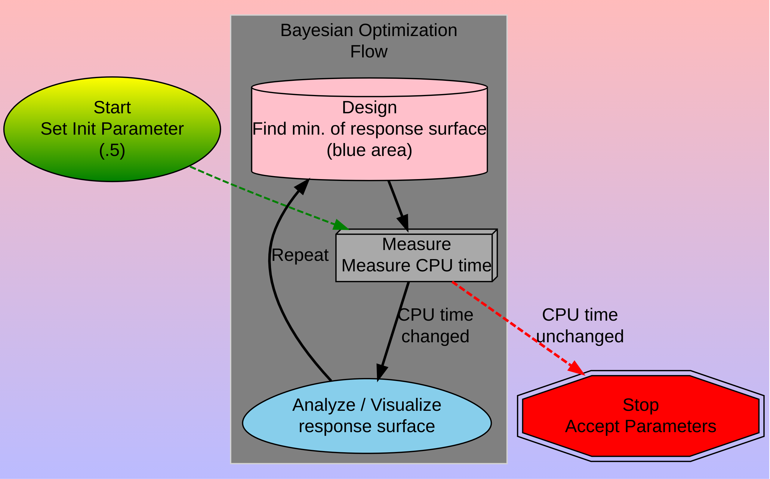
Bayesian Optimization Flow
Single Parameter
What do we know about the system?
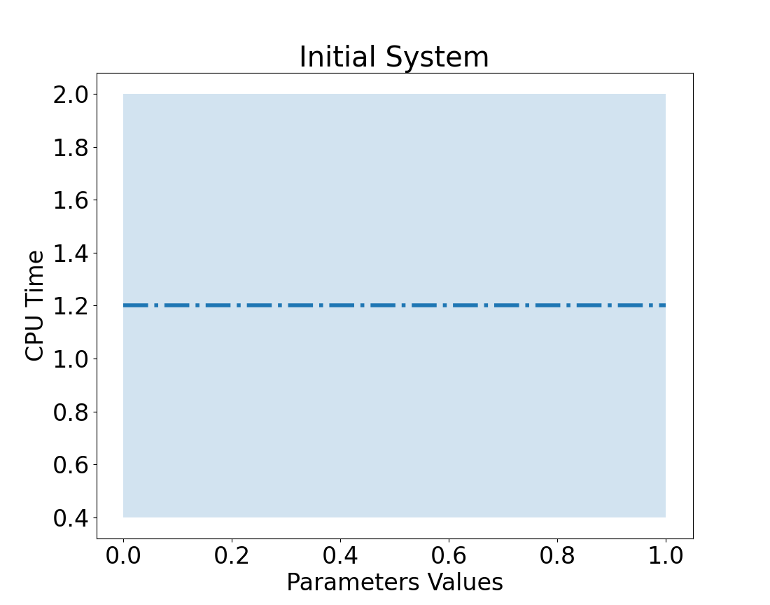
Our system
Single parameter: bounded between 0 - 1
Current CPU run time: 1.2 hours
Seen system take over 2 hours
Uncertainty, is constant
We have not made a measurement!
So we do not know how the system will respond.
We could make it worse or better.
Look, we have a response surface! (shaded blue area)
Let’s take a measurement.
What measurement should we take first?
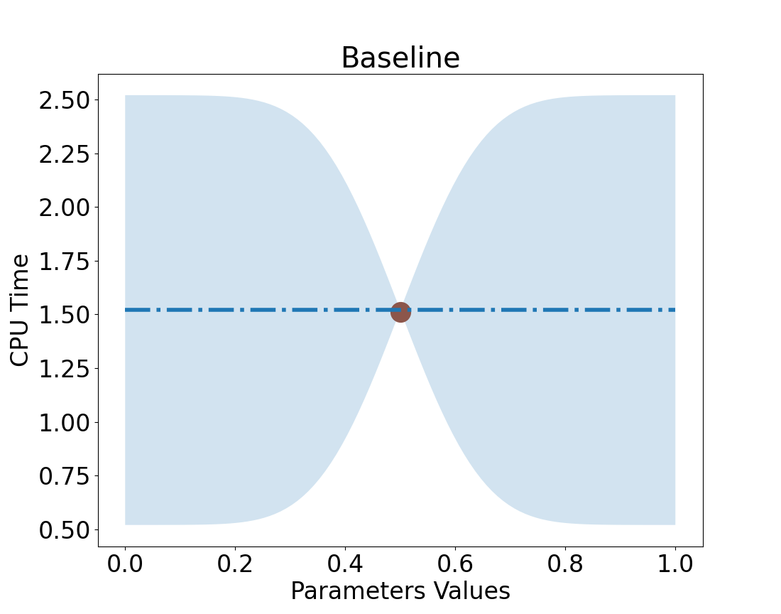
Let’s take a value in the middle.
Value = 0.5
Run CPU test.
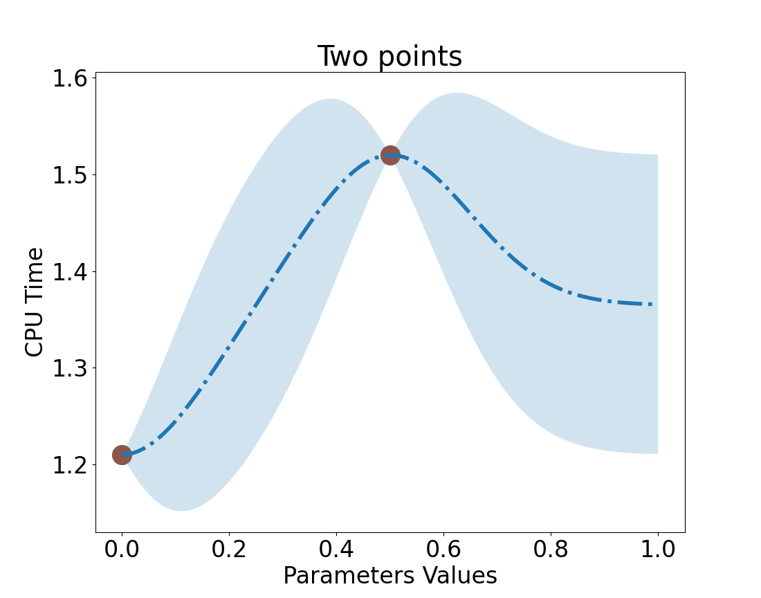
Which results in
CPU Time is ~1.5
So, what happens to our uncertainty.
near value = 0.5?
near 0?
near 1?
Take a measurement
Note: Uncertainty follows an exponential decay: \(exp(-x^2)\)
Now what,
How do we decide on which point to take next?
Pick a point that has the highest uncertainty!
We want to reduce uncertainty.
Let’s make another measurement.
Pick, Value = 0
We could have chosen 1 too.
Run CPU Test
Result = ~1.2
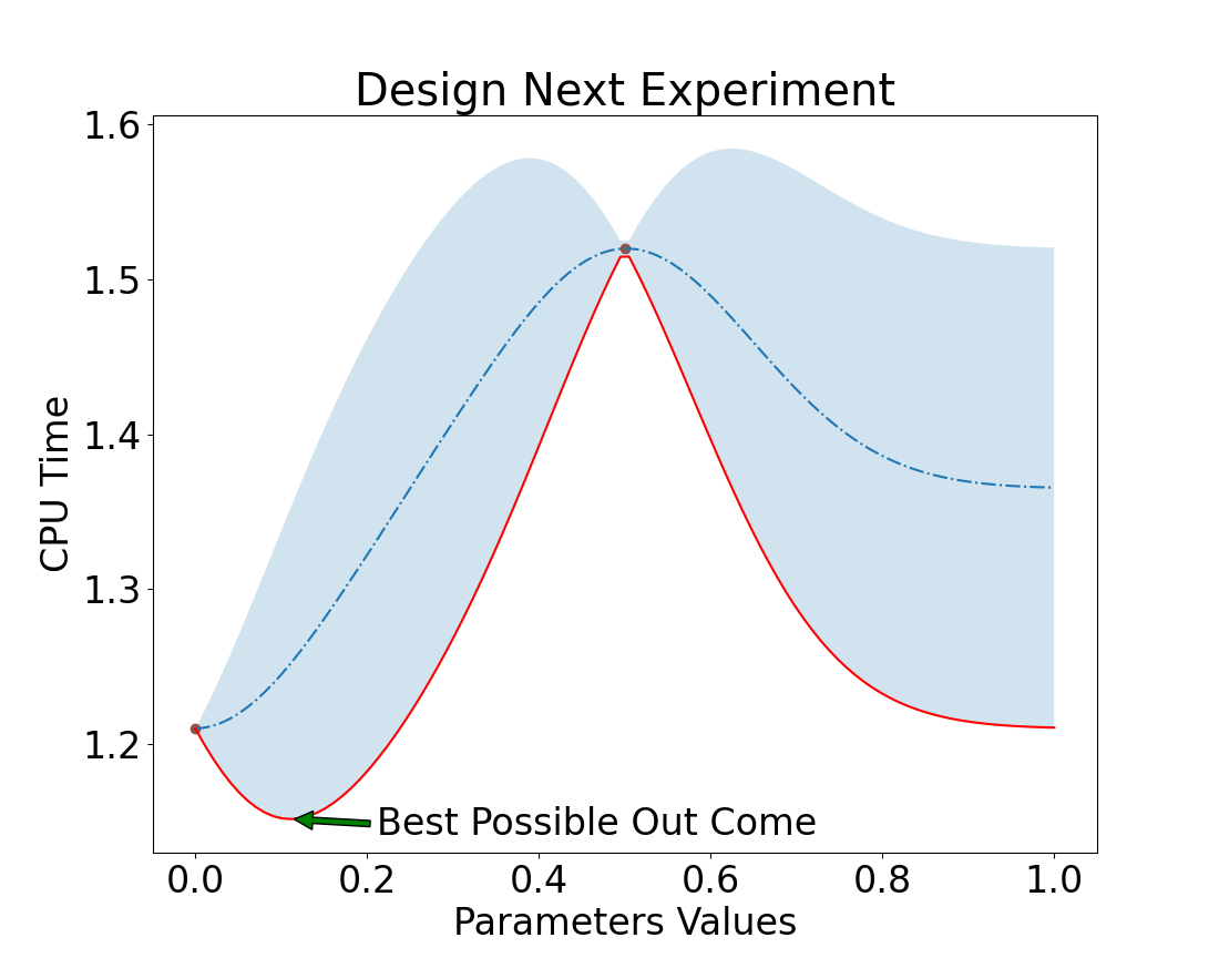
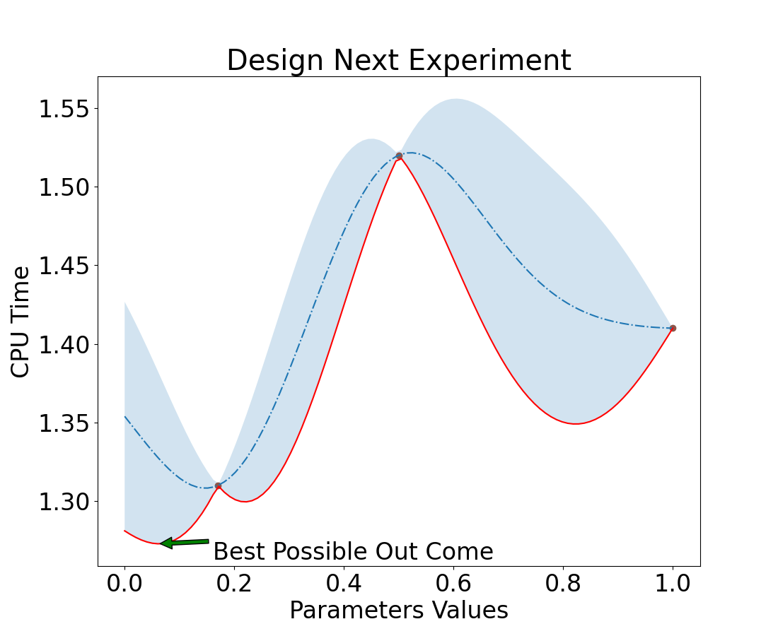
Design next Experiment
We want to pick a value that lowers uncertainty but,
has the best expected outcome.
Focus on the Goal
Remember our goal is to make the website faster.
Nice, but how did you make that response surface?
The shaded area is our uncertainty times the standard deviation of results (y).
\(uncertainty * \sigma_y\)
How is uncertainty calculated?
def kernel(self, x1, x2):# find the distance between a measured and unmeasured point# Want to weight points near a measured one more distance_squared = ((x1-x2)**2)return np.exp(-distance_squared/(2*self.sigma**2))def estimate(self, query_parameter): kernels_x_query = np.array([self.kernel(x, query_parameter)for x inself.x]) kernels_x_x = np.array([[self.kernel(x1, x2) for x1 inself.x]for x2 inself.x]) weights= kernels_x_query.T @ np.linalg.inv(kernels_x_x) expectation =self.mean_y + weights @self.y # Dashed line uncertainty_squared =1- weights @ kernels_x_query uncertainty = np.sqrt(uncertainty_squared)return expectation, self.std_y*uncertainty
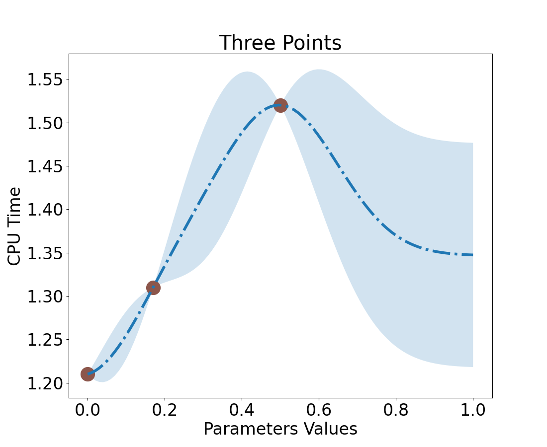
Run the experiment
Value = .17
import bo_scripts as bo# GPR is Gaussian Processes Responsex = [0.5, 0.0, ]y = [1.52, 1.21]sigma =.5gpr = bo.GPR4(x, y, sigma)x_hat =0.17# Our value y_hat, uncertainty = gpr.estimate(x_hat) print(f"y_hat is {round(y_hat,2)} with uncertainty={round(uncertainty,2)}")
y_hat is 1.31 with uncertainty=0.02
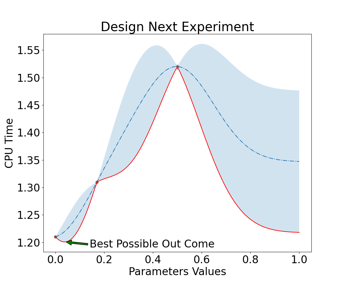
Resulting in a new response surface
Converging to Optimal Solution
We can see that we are converging quickly to an optimal solution
If Second Measure had value 0 or 1
Remember we chose 0 to be our second value. We still get the same solution.
Value = 0
Value = 1
Now Multi Variables
This is where the fun begins.
Given
Our CPU test takes 1 hour and we want to sample each variable 10 times.
How long would it take to run this experiment.
10 * 10 * 10 * 10 * 10 * 10 * 10
\(10^7\)
~ 417,000 days
In 1000 years no one is going to care about your website.
So how do we improve the website while the content is still current?
Random Search
Wait!!!!!
What,
How is this different than Monte Carlo Method
Monte Carlo method is similar in a sense that we randomly select values to run our experiment.
However, in Bayesian Optimization we feed in past results and model the response surface to know if we are moving in the right direction.
We can see how the systems is converging to an optimized solution.
BO with Random Search
Generate our next design experiment by adding (small) random number to each value in your vector
Evaluate this new vector of parameters
Compare old and new vector results, take best.
Repeat
BO with Random Search
Ask
Calculate the response curve and find the low confidence band (LCD)
Spend some time looking for the new vector to try, via estimates.
Each iteration we estimate our expectation.
Test if lcb is lower with the new vector
Repeat 200 times
Export the best vector
Tell
Actually run the experiment (~1 hour)
Append measurements
Lastly
Repeat for 2 days (48 runs)
Note: It will take longer to calculate the estimates, when the number of measurements increase.
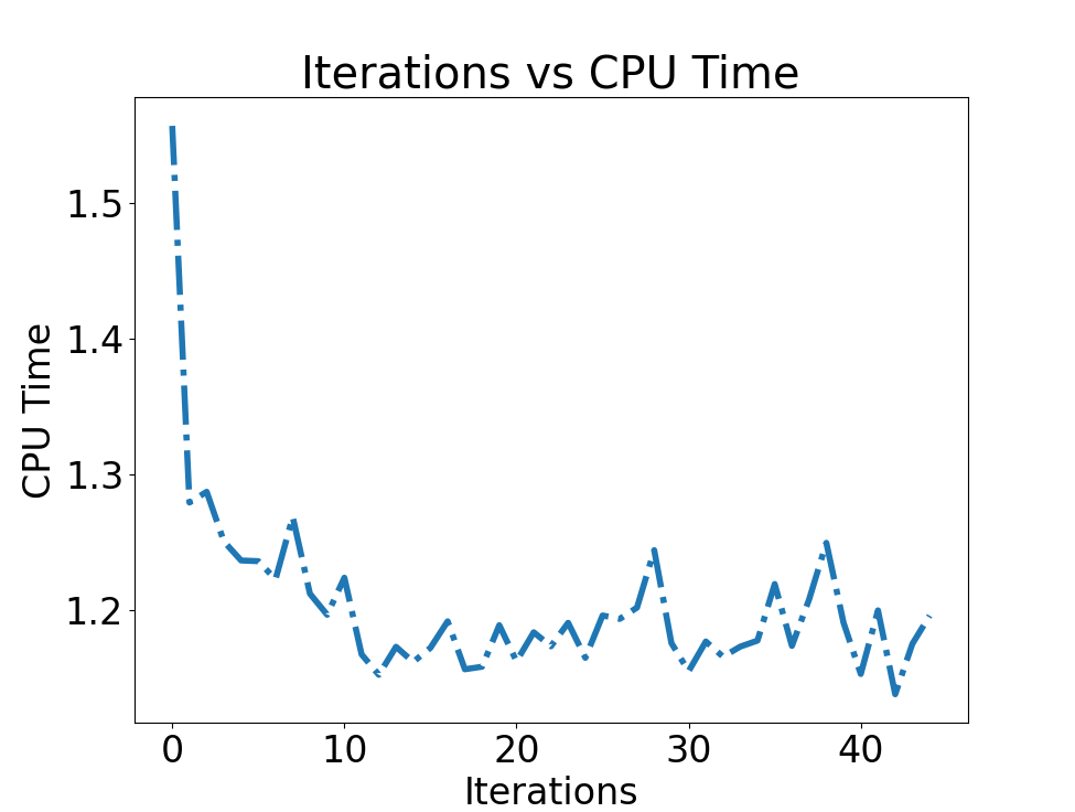
BO Results
Lets look at the code.
Thank you
Thank you
We optimized a system that would have took us over 1000 years to a couple days!