Linear Algebra for ML/AI aka Green AI

Welcome

Presented by Evelyn J. Boettcher

2023-10-19

Ax-b = 0

System of Linear Equations

Solving a system of linear equations is fast.

It can easily and quickly handle large data.

So if you can get your problems into the Ax=b form; your golden.

Ax=b, in action

System of linear equations

3x + 4y = 19
2y + 3z = 8
4x - 5z = 7

In Matrix form

\[ A = \begin{bmatrix} 3 & 4 & 0\\ 0 & 2 & 3 \\ 4 & 0 & -5 \end{bmatrix} \]

\[ b = \begin{bmatrix} 19 \\ 8\\ 7 \end{bmatrix} \]

\[ A = \begin{bmatrix} 3 & 4 & 0\\ 0 & 2 & 3 \\ 4 & 0 & -5 \end{bmatrix} \]

\[ b = \begin{bmatrix} 19 \\ 8\\ 7 \end{bmatrix} \]

Solve with python

import numpy as np
A = np.array([[3, 4, 0],
              [0, 2, 3], 
              [4, 0, -5]])
B = np.array([19, 8, 7])
# Using np built-in linear equation solver
x = np.linalg.solve(A,B)
print( tuple(x))
# WOW that was easy.

(3.0, 2.5, 1.0)

What if you don’t have a “Full Rank” matrix

Or systems that can be fulled solved?

This is where SVD (Single Value Decomposition) comes to the rescue.

Beyond solving a system of linear equations.

It is used for:

It is used to compress images
Find main features (see compressed images)
for fitting Polynomial.
Predict Sun spots activity

As long as you can get your problem into the Ax=b form.

SVD

Singular value decomposition (SVD) is a factorization of a real or complex matrix.

SVD of Matrix A is:

SVD(A) = \(U \Sigma V^T\)

So when we system that can be written as: Ax=b

We can solve for x by:

\[ x^\prime = V \Sigma U^T b \]

Then \(x^\prime\) is the solution that has the minimum norm (closest to origin). If it is not in the range, then it is the least-squares solution.

Wow that was clear.

Take a minute and google how to multiply matrixs

Great resource: SVD Tutorial

Sun Spots predictions

There exists a data set that contains the number of sun spots observed for a given month, spanning hundreds of years.

https://github.com/ejboettcher/GemCity-ML-AI_Random

In the above tutorial, I used tensorflow, WITH GPU and it took several minutes to train the algorithm to predict sunspot activity. And it was good.

Can SVD predict sunspot activity and faster?

Blindly use an SVD

import numpy as np
import matplotlib.pyplot as plt
import pandas as pd

sunspot_data = pd.read_csv("data/Sunspots.csv")
sunspot_data['time'] = pd.to_datetime(sunspot_data['Date'], format='%Y-%m-%d')
nname = 'Monthly Mean Total Sunspot Number'

window = 1
dataset = np.ones((len(sunspot_data)-window, window))
for ii in range(len(dataset)):
    dataset[ii,:] = sunspot_data.loc[ii:ii+window-1, nname].to_numpy().T

A = dataset
A = np.column_stack([np.ones(A.shape[0]), A])
b = sunspot_data.loc[window:, nname].to_numpy()

# calculate the economy SVD for the data matrix A
U,S,Vt = np.linalg.svd(A, full_matrices=False)

# solve Ax = b for the best possible approximate solution in terms of least squares
x_hat = Vt.T @ np.linalg.inv(np.diag(S)) @ U.T @ b

# perform train and test inference
b_pred = A @ x_hat

train_data = pd.DataFrame({'time':sunspot_data.loc[window:,'time'],
                           'b':b, 
                           'b_pred':b_pred} )
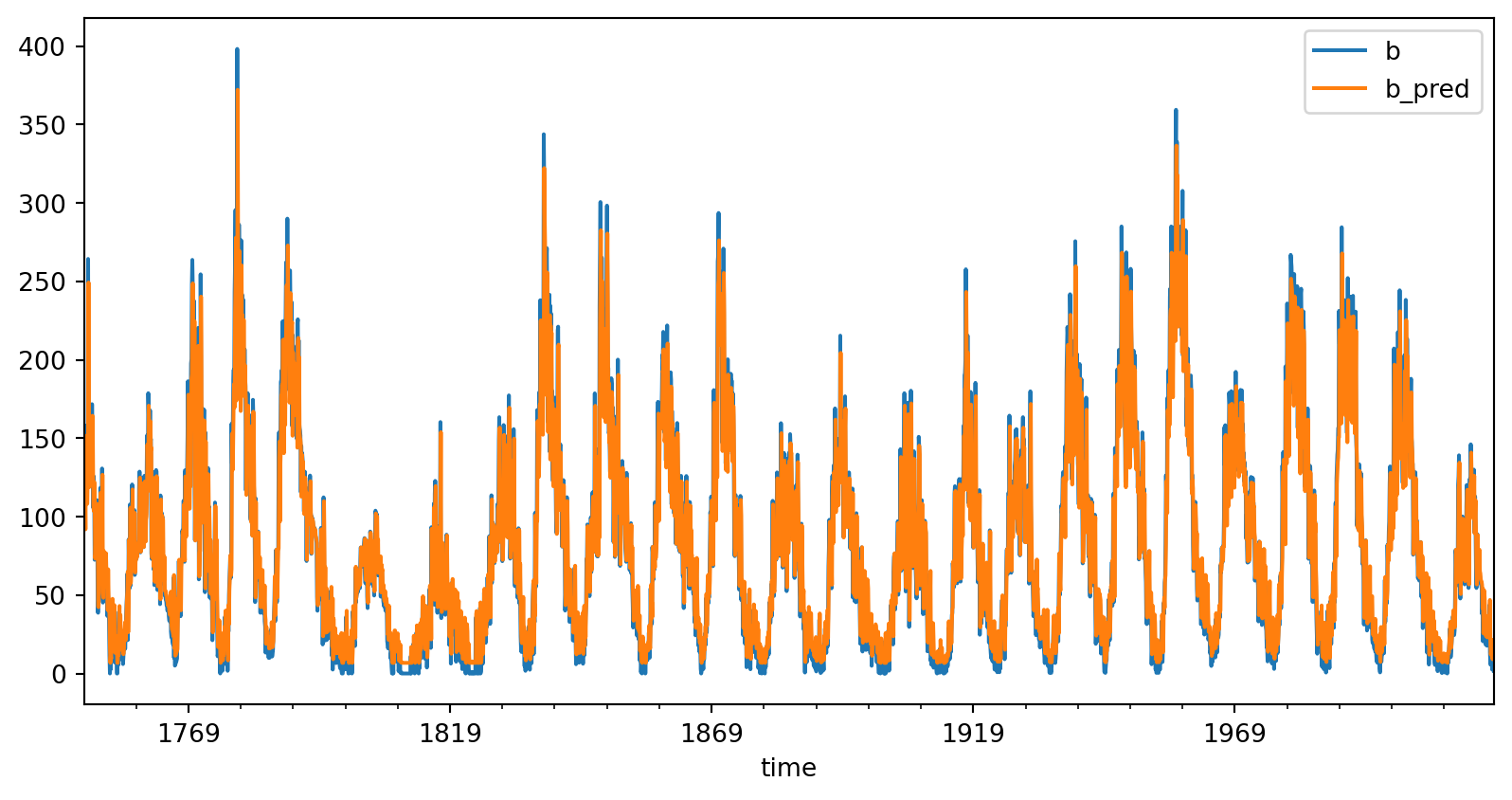
train_data.plot(x='time', y=['b', 'b_pred'])

# compute train and test MSE
train_mse = np.mean(np.sqrt((b_pred - b)**2))
print("Train Mean Squared Error:", train_mse)
plt.show()

Train Mean Squared Error: 19.273508962865446

More features

import numpy as np
import matplotlib.pyplot as plt
import pandas as pd

sunspot_data = pd.read_csv("data/Sunspots.csv")
sunspot_data['time'] = pd.to_datetime(sunspot_data['Date'], format='%Y-%m-%d')
nname = 'Monthly Mean Total Sunspot Number'

window = 12
dataset = np.ones((len(sunspot_data)-window, window))
for ii in range(len(dataset)):
    dataset[ii,:] = sunspot_data.loc[ii:ii+window-1, nname].to_numpy().T

A = dataset
A = np.column_stack([np.ones(A.shape[0]), A])
b = sunspot_data.loc[window:, nname].to_numpy()

# calculate the economy SVD for the data matrix A
U,S,Vt = np.linalg.svd(A, full_matrices=False)

# solve Ax = b for the best possible approximate solution in terms of least squares
x_hat = Vt.T @ np.linalg.inv(np.diag(S)) @ U.T @ b

# perform train and test inference
b_pred = A @ x_hat

train_data = pd.DataFrame({'time':sunspot_data.loc[window:,'time'],
                           'b':b, 
                           'b_pred':b_pred} )
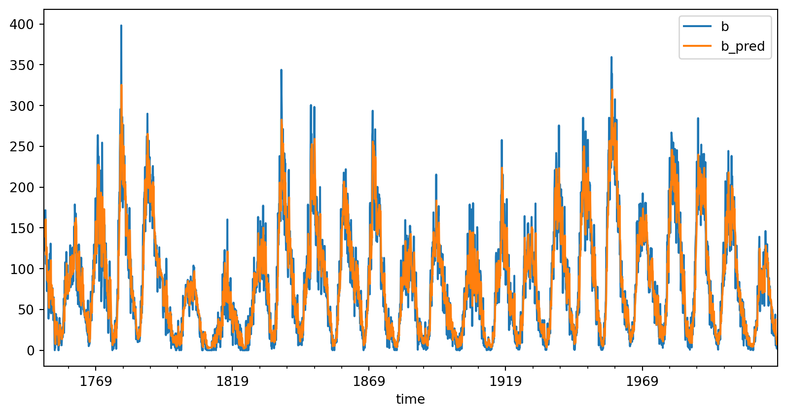
train_data.plot(x='time', y=['b', 'b_pred'])

# compute train and test MSE
train_mse = np.mean(np.sqrt((b_pred - b)**2))
print("Train Mean Squared Error:", train_mse)
plt.show()

Train Mean Squared Error: 17.875197212239335

Prove it on data it has not seen.

split_num = 3000
A = dataset
A = np.column_stack([np.ones(A.shape[0]), A])
X_train = A[:split_num,:]
y_train = sunspot_data.loc[window:split_num+window-1, nname].to_numpy()

X_test = A[split_num:,:]
y_test = sunspot_data.loc[split_num+window:, nname].to_numpy()

print(X_test.shape, y_test.shape, X_train.shape, y_train.shape)
# calculate the economy SVD for the data matrix A
U,S,Vt = np.linalg.svd(X_train, full_matrices=False)

# solve Ax = b for the best possible approximate solution in terms of least squares
x_hat = Vt.T @ np.linalg.inv(np.diag(S)) @ U.T @ y_train

# perform train and test inference
y_pred = X_train @ x_hat
test_predictions = X_test @ x_hat  # This is the MAGIC

test_data =  pd.DataFrame({'time':sunspot_data.loc[split_num+window:,'time'],
                           'test':y_test, 
                           'y_pred':test_predictions} )
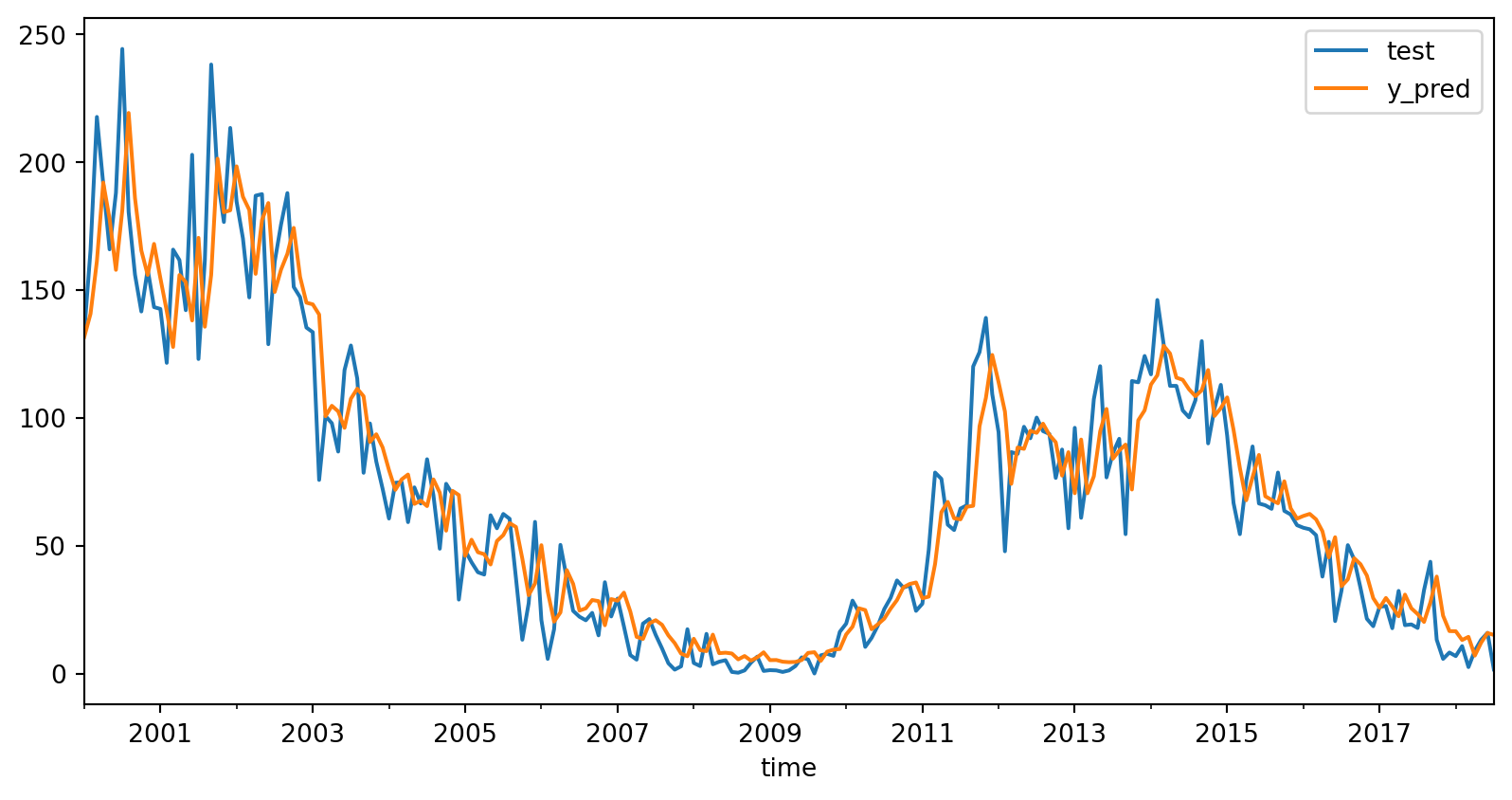
test_data.plot(x='time', y=['test', 'y_pred'])


# compute train and test MSE
train_mse = np.mean(np.sqrt((y_pred - y_train)**2))
test_mse = np.mean(np.sqrt((test_predictions - y_test)**2))

print("Train Mean Squared Error:", train_mse)
print("Test Mean Squared Error:", test_mse)
plt.show()

(223, 13) (223,) (3000, 13) (3000,)
Train Mean Squared Error: 18.20793849887562
Test Mean Squared Error: 13.688869408003756

?

What

Explain again what an SVD does.

Let’s take a look at how SVD can be used for image compression.

tutorial

Thank you

SVD can just do it. You just need to get it into the Ax=B form.